Kakakuona Forum

What is pre-trained Models ???

A pre-trained model is a machine learning (ML) model that has been trained on a large dataset and can be fine-tuned for a specific task. as defined by encord.
Or
A pretrained AI model is a deep learning model that’s trained on large datasets to accomplish a specific task, and it can be used as is or customized to suit application requirements across multiple industries.
as defined by nvidia blog

A pre-trained AI model is a deep learning model, which made by comparing how neural work on human brain, which used to find patterns in data or make prediction based on given data.

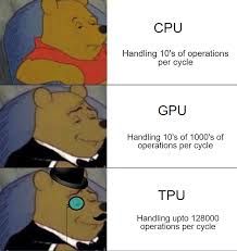
Recently after improve in hardware and introducing of very powerful processor (CPU (Central Processing Unit), GPU (Graphics Processing Unit), and TPU (Tensor Processing Unit) )

CPU: General-purpose processing.
GPU: Parallel processing, primarily for graphics and scientific computing.
TPU: Specialized processing for machine learning tasks.

The TPU is a type of processor developed by Google specifically for accelerating machine learning workloads. It can be used through Google Clouds service. TPU can be most useful over all other when it come neural/deep learning because It is optimized for performing tensor operations, which are the backbone of many machine learning algorithms, especially those involving neural networks.
even though GPU can be useful but thats another day lesson...

Lets continue with pre-trained models

WHY PRE-TRAINED MODELS ??
Pre-trained models can be useful for developers and researchers because they can save time and resources, and can be just as effective as custom models. In trainings model there are different problem we face first datasets, resource and last time let take a simple example of BERT model

Resource	Model	Time Used to Train
TPU (16 chips)	BERT-Base	4 days
TPU (64 chips)	BERT-Large	4 days

you can see how long it take to train model and how much of resource used it hard to stand this math, For small developers and researchers so pre trained model was released in order to save time and resources used in training models from scratch. Now big pre trained models like gpt-2, BERT, gemma2, ELMo, Transformer-XL, and RoBERTa,VGG, ResNet, and Inception have been released and now researchers can save steps and start building from certain point not from scratch so what we have is a models taught everything at generally like gpt-2, and BERT, and we come with specific datasets and fine-tune the model using our datasets so it can be useful in specific area

DISADVANTAGE OF PRE-TRAINED MODEL

Domain-Specific Features: Pretrained models are often trained on large and diverse datasets, but they may not capture domain-specific features relevant to your specific task

Overfitting: If the pretrained model is very large and your dataset is relatively small, there's a risk of overfitting. The model may memorize the training data rather than learning generalizable patterns.

Lack of Transparency: Pretrained models are often black boxes, making it challenging to understand how they make predictions. This lack of transparency can be problematic in applications where interpretability and explainability are important.

Pre-existing biases in pre-trained models can arise from the data they were originally trained on. Most pre-trained models, like BERT or GPT, were trained primarily on large English datasets. This can create several issues, especially when trying to use these models for languages like Swahili.

Prepared By Alfred Baraka
Computer Science Student
Data Science Enthusiast

HOW TO KNOW WHICH NUMBER OF COMPONENTS IS GOOD

On above documentary i explain to you about PCA but i did not tell you exactly how we choose number of components for PCA if we choose wrong number of component there will be higher variance difference and we can lead to wrong model Teaching.

Lets say we have our array and we dont know exactly how many number of components can be useful so then we apply explained_variance ratio concept

from sklearn.decomposition import PCA

pca = PCA()
new_feature = pca.fit_transform(array)
np.var(new_feature)
pca.explained_variance_ratio_

Return

array([0.92461872, 0.05306648, 0.01710261, 0.00521218])

And after that we apply cumulative sum to make our data visual presented

pca.explained_variance_ratio_
cumsum = np.cumsum(pca.explained_variance_ratio_)
cumsum

Return

array([0.92461872, 0.97768521, 0.99478782, 1.        ])

And then Plotting

plt.plot(cumsum)
plt.axhline(y=0.97, c='r', linestyle='-')
plt.grid(True)
plt.show()

After that we manually inspect to found best number of component that will save original Data Variance by 97%

d = np.argmax(cumsum > 0.97) + 1
print(d)

Return

2

So thats how we choose n_component = 2 and saave model efficiency at the same time

What is PCA ??
According to builtin Website "Principal component analysis (PCA) is a dimensionality reduction and machine learning method used to simplify a large data set into a smaller set while still maintaining significant patterns and trends."

Two Important Keys Found Here

• dimensionality reduction : a method for representing a given dataset using a lower number of features (i.e. dimensions) while still capturing the original data's meaningful properties

• patterns recognizable sequences of data points that have a consistent structure.

Sometimes in machine learning we face huge amount of data like data that Contain millions of row and hundreds of column. Maybe large amount of data in dataset can help us to made very efficiency and powerful model???, True but we need many records/data/row and not many columns

Having many columns in a dataset, known as high dimensionality, can lead to several challenges in machine learning. It increases computational costs and training time, complicates the feature selection process, and raises the risk of overfitting due to the "curse of dimensionality." Additionally, high dimensionality can result in multicollinearity(Multicollinearity is a statistical concept where several independent variables in a model are correlated), where highly correlated features distort the model's understanding of individual feature contributions, making the model harder to interpret. These issues can hinder the model's performance and its ability to generalize well to new data.

We will use a practical hands-on approach to understand the algorithms. using Iris datasets that are found in scikit-learning library datasets

We will start by importing important library

import sklearn.datasets
import numpy as np
import matplotlib.pyplot as plt
import pandas as pd
from sklearn.preprocessing import StandardScaler

After that then we will load our data as Iris

Iris = sklearn.datasets.load_iris()
Iris

Return

{'data': array([[5.1, 3.5, 1.4, 0.2],
        [4.9, 3. , 1.4, 0.2],
        [4.7, 3.2, 1.3, 0.2],
        [4.6, 3.1, 1.5, 0.2],
        [5. , 3.6, 1.4, 0.2],
.............
'petal length (cm)',
  'petal width (cm)'],
 'filename': '/home/egovridc/.local/lib/python3.6/site-packages/sklearn/datasets/data/iris.csv'}

We can show how data in tabular format like:

df_Iris_data = pd.DataFrame(Iris.data, columns= Iris.feature_names)
df_Iris_target = pd.DataFrame(Iris.target, columns=['Species'])
df_Iris = pd.concat([df_Iris_data, df_Iris_target], axis=1)
df_Iris.head()

Return

And Statistical info of our data is

df_Iris.describe()

So know we have our data, We learn it and we understand it well, Then Whats next??

PCA
Consider we have x = [Sepallength, SepalWidth, PetalLength, Petalwidth] and we should use it to predict the value of y which which can be 'setosa', 'versicolor', 'virginica'

So question come do we need all four features in order to know the species of the flower, Or do we only need 3 or 2 features??

Lets think !!!
If we have a few features our model prediction Performance will be higher.
But if we drop Important feature Our model efficiency will be very Low...
Then what we done...??

Then here we apply Dimension Reduction

Even though we should understand Dimension reduction come with its advantage like less interpretability of the transformed features and loss of details due to feature elimination, Am i confuse you?? Wait take deep breath lets code and from our final result we can understand why less interpretability and loss of details

Theoretically PCA is a Unsupervised Learning remind you the definition of unsupervised Learning
also known as unsupervised machine learning, uses machine learning (ML) algorithms to analyze and cluster unlabeled data sets. These algorithms discover hidden patterns or data groupings without the need for human intervention. as defined by IBM Website

As we mentioned before, the goal of PCA is to reduce the number of features by projecting them into a reduced dimensional space constructed by mutually orthogonal features (also known as “principal components”) with a compact representation of the data distribution.

Up to now i think you comprend moi as French Said...

And now we will Perform few others step to accomplish PCA start by convert our data to array after that Standardize our data

df_Iris
array = np.array(df_Iris.iloc[:, :-1])
array

Return

array([[5.1, 3.5, 1.4, 0.2],
       [4.9, 3. , 1.4, 0.2],
.....
[6.2, 3.4, 5.4, 2.3],
       [5.9, 3. , 5.1, 1.8]])

Data Standardization

sc = StandardScaler()
Standardized_feature = sc.fit_transform(array)
Standardized_feature

Return

array([[-9.00681170e-01,  1.01900435e+00, -1.34022653e+00,
        -1.31544430e+00],
......
[ 4.32165405e-01,  7.88807586e-01,  9.33270550e-01,
         1.44883158e+00],
       [ 6.86617933e-02, -1.31979479e-01,  7.62758269e-01,
         7.90670654e-01]])

Apply PCA

from sklearn.decomposition import PCA
pca = PCA(n_components=2)
reduced_feature = pca.fit_transform(Standardized_feature)
reduced_feature

Return

# We success reduced feature from 4 to 2 and retain its pattern
array([[-2.26470281,  0.4800266 ],
       [-2.08096115, -0.67413356],
.........
[ 1.37278779,  1.01125442],
       [ 0.96065603, -0.02433167]])

But Wait!!!
Remember the disadvantage now we cannot interprete new features but we can use on model and having better Performance than ever

Prepared By Alfred Baraka
Computer Science Student
Data Science Enthusiast