Performing Principle Component Analysis, Why and How ??
-
What is PCA ??
According to builtin Website "Principal component analysis (PCA) is a dimensionality reduction and machine learning method used to simplify a large data set into a smaller set while still maintaining significant patterns and trends."Two Important Keys Found Here
-
dimensionality reduction : a method for representing a given dataset using a lower number of features (i.e. dimensions) while still capturing the original data's meaningful properties
-
patterns recognizable sequences of data points that have a consistent structure.
Sometimes in machine learning we face huge amount of data like data that Contain millions of row and hundreds of column. Maybe large amount of data in dataset can help us to made very efficiency and powerful model???, True but we need many records/data/row and not many columns
Having many columns in a dataset, known as high dimensionality, can lead to several challenges in machine learning. It increases computational costs and training time, complicates the feature selection process, and raises the risk of overfitting due to the "curse of dimensionality." Additionally, high dimensionality can result in multicollinearity(Multicollinearity is a statistical concept where several independent variables in a model are correlated), where highly correlated features distort the model's understanding of individual feature contributions, making the model harder to interpret. These issues can hinder the model's performance and its ability to generalize well to new data.

We will use a practical hands-on approach to understand the algorithms. using Iris datasets that are found in scikit-learning library datasets
We will start by importing important library
import sklearn.datasets
import numpy as np
import matplotlib.pyplot as plt
import pandas as pd
from sklearn.preprocessing import StandardScaler
After that then we will load our data as Iris
Iris = sklearn.datasets.load_iris()
Iris
Return
{'data': array([[5.1, 3.5, 1.4, 0.2],
        [4.9, 3. , 1.4, 0.2],
        [4.7, 3.2, 1.3, 0.2],
        [4.6, 3.1, 1.5, 0.2],
        [5. , 3.6, 1.4, 0.2],
.............
'petal length (cm)',
  'petal width (cm)'],
 'filename': '/home/egovridc/.local/lib/python3.6/site-packages/sklearn/datasets/data/iris.csv'}
We can show how data in tabular format like:
df_Iris_data = pd.DataFrame(Iris.data, columns= Iris.feature_names)
df_Iris_target = pd.DataFrame(Iris.target, columns=['Species'])
df_Iris = pd.concat([df_Iris_data, df_Iris_target], axis=1)
df_Iris.head()
Return
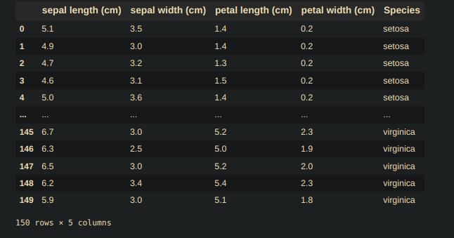
And Statistical info of our data is
df_Iris.describe()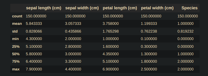
So know we have our data, We learn it and we understand it well, Then Whats next??

PCA
Consider we have x = [Sepallength, SepalWidth, PetalLength, Petalwidth] and we should use it to predict the value of y which which can be 'setosa', 'versicolor', 'virginica'So question come do we need all four features in order to know the species of the flower, Or do we only need 3 or 2 features??
Lets think !!!
If we have a few features our model prediction Performance will be higher.
But if we drop Important feature Our model efficiency will be very Low...
Then what we done...??Then here we apply Dimension Reduction
Even though we should understand Dimension reduction come with its advantage like less interpretability of the transformed features and loss of details due to feature elimination, Am i confuse you?? Wait take deep breath lets code and from our final result we can understand why less interpretability and loss of details
Theoretically PCA is a Unsupervised Learning remind you the definition of unsupervised Learning
also known as unsupervised machine learning, uses machine learning (ML) algorithms to analyze and cluster unlabeled data sets. These algorithms discover hidden patterns or data groupings without the need for human intervention. as defined by IBM WebsiteAs we mentioned before, the goal of PCA is to reduce the number of features by projecting them into a reduced dimensional space constructed by mutually orthogonal features (also known as “principal components”) with a compact representation of the data distribution.
Up to now i think you comprend moi as French Said...
And now we will Perform few others step to accomplish PCA start by convert our data to array after that Standardize our data
df_Iris
array = np.array(df_Iris.iloc[:, :-1])
array
Return
array([[5.1, 3.5, 1.4, 0.2],
       [4.9, 3. , 1.4, 0.2],
.....
[6.2, 3.4, 5.4, 2.3],
       [5.9, 3. , 5.1, 1.8]])
Data Standardization
sc = StandardScaler()
Standardized_feature = sc.fit_transform(array)
Standardized_feature
Return
array([[-9.00681170e-01,  1.01900435e+00, -1.34022653e+00,
        -1.31544430e+00],
......
[ 4.32165405e-01,  7.88807586e-01,  9.33270550e-01,
         1.44883158e+00],
       [ 6.86617933e-02, -1.31979479e-01,  7.62758269e-01,
         7.90670654e-01]])
Apply PCA
from sklearn.decomposition import PCA
pca = PCA(n_components=2)
reduced_feature = pca.fit_transform(Standardized_feature)
reduced_feature
Return
# We success reduced feature from 4 to 2 and retain its pattern
array([[-2.26470281,  0.4800266 ],
       [-2.08096115, -0.67413356],
.........
[ 1.37278779,  1.01125442],
       [ 0.96065603, -0.02433167]])
But Wait!!!
Remember the disadvantage now we cannot interprete new features but we can use on model and having better Performance than everPrepared By Alfred Baraka
Computer Science Student
Data Science Enthusiast -
-
HOW TO KNOW WHICH NUMBER OF COMPONENTS IS GOOD
On above documentary i explain to you about PCA but i did not tell you exactly how we choose number of components for PCA if we choose wrong number of component there will be higher variance difference and we can lead to wrong model Teaching.
Lets say we have our array and we dont know exactly how many number of components can be useful so then we apply explained_variance ratio concept
from sklearn.decomposition import PCA

pca = PCA()
new_feature = pca.fit_transform(array)
np.var(new_feature)
pca.explained_variance_ratio_
Return
array([0.92461872, 0.05306648, 0.01710261, 0.00521218])And after that we apply cumulative sum to make our data visual presented
pca.explained_variance_ratio_
cumsum = np.cumsum(pca.explained_variance_ratio_)
cumsum
Return
array([0.92461872, 0.97768521, 0.99478782, 1. ])And then Plotting
plt.plot(cumsum)
plt.axhline(y=0.97, c='r', linestyle='-')
plt.grid(True)
plt.show()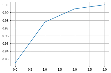
After that we manually inspect to found best number of component that will save original Data Variance by 97%
d = np.argmax(cumsum > 0.97) + 1
print(d)
Return
2So thats how we choose n_component = 2 and saave model efficiency at the same time